SUSPENSION TUNING MODULE (STM)
|
|
The DYNATUNE-XL SUSPENSION TUNING MODULE is an ulterior standalone Module with significant Enhancements over te Standard Ride Feature Tool of the DYNATUNE-XL R&H MODULE. In DYNATUNE_XL STM do exist interactions between Front & Rear Body and Non-Linear Damping and (from RELEASE 8.1 onward) Non-Linear Spring Rates are more accurately represented by instantaneous Force-Velocity Maps resp. Force-Displacements Maps.
Furthermore since RELEASE 8.0.1, a truly unique DAMPER CURVE CREATION & OPTIMIZATION Procedure does allow the User to create Damper Characteristics which meet specific requirements for Body Damping, Wheel Control and Comfort Perception within minutes. |
STM features a "Control Section Panel" that includes user-friendly Scaling Factors for Spring Rates and Damper Jounce & Rebound Force-Velocity Curves, facilitating rapid optimization cycles in line with the DYNATUNE-XL Philosophy of maximizing results with minimal input data.
Built as a standard MS EXCEL ® workbook, the tool leverages both standard workbook functions and custom-written VBA code for live Fast Fourier Transformation in the Frequency Transfer Function Algorithm.
NOTE: DYNATUNE SUSPENSION TUNING MODULE (STM) IS NOT INCLUDED IN ANY OTHER DYNATUNE TOOL. IT COMES AS A STANDALONE TOOL ONLY.
|
Straight Out of the Box Damper Setting
|
Setup comparison between competitors
|
A picture tells more than a Thousand Words
|
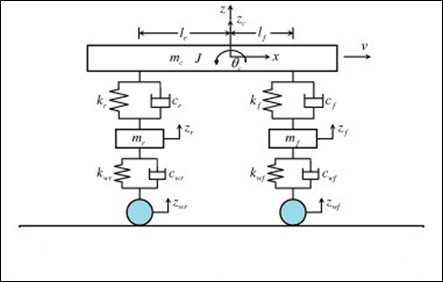
Analytical MODEL
|
The DYNATUNE STM Fully Dynamic Ride Model is used for numerically calculating the response of the vehicle to a road input signal. It consists of a 4 DOF / 3 PART (bicycle) model with a Sprung Body, Unsprung Masses, and Springs & (Non-Linear) Dampers.
The Sprung Mass is connected to Front & Rear Spring & Damper systems. Wheels are connected to the ground, each via a Tire Spring and Tire Damping (calculated from the critical tire damping input parameter). The differential equations of motion are solved in the time domain through numerical integration/differentiation with a 0.001 s. step size. |
|
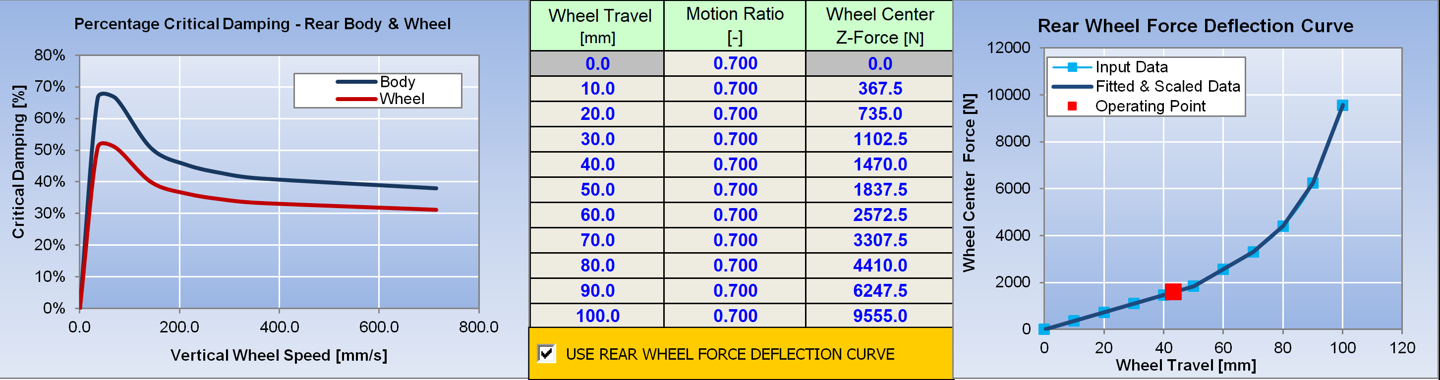
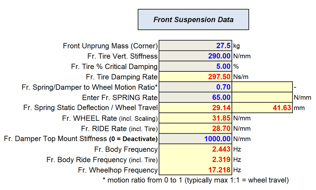
RELEASE 8.1 - SPRiNG INPUT DATA - NON-LiNEAR WHEEL DEFLECTION CURVE
Starting from RELEASE 8.1, it is now possible to specify not only a linear spring rate but also a Non-Linear Wheel Force Deflection Curve and, if desired, a Non-Linear Motion Ratio Curve. This enhancement enables the combination of various suspension wheel rate configurations.
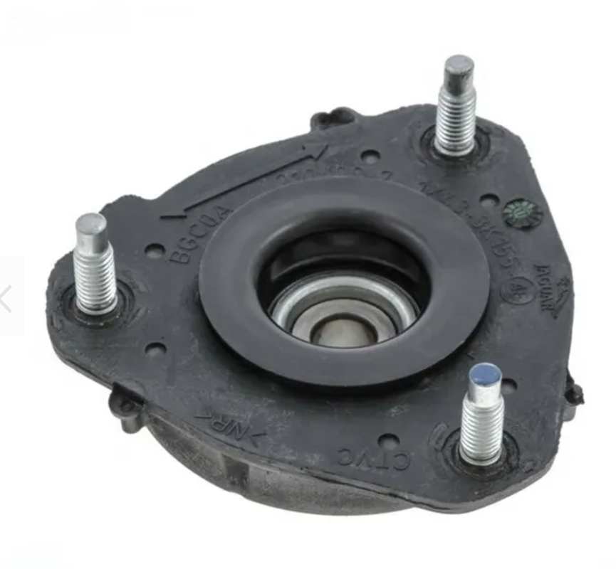
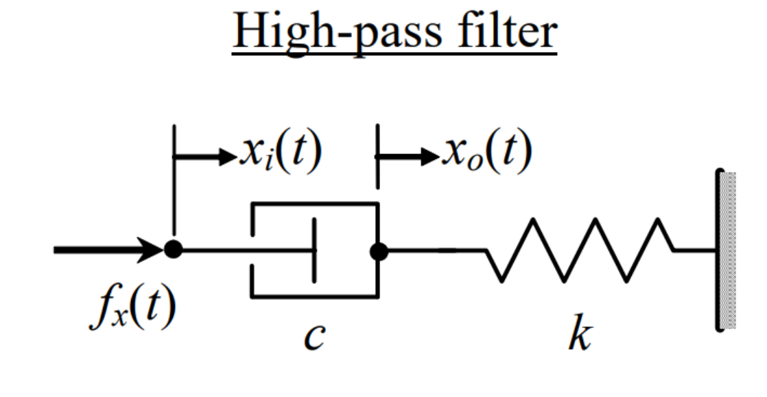
In addition to the Vertical Wheel Force Deflection Curve, the user now has the option to implement a Damper Top Mount, commonly found in many OEM applications. This top mount, to which a Damper Unit is attached, effectively couples a Damper and a Spring in Series, creating an additional mechanical equivalent of a High Pass Filter. This feature is often utilized for improving ride comfort and filtering.
|
|
|
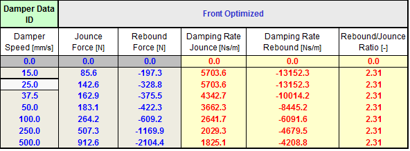
DAMPER INPUT DATA
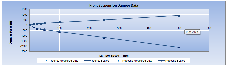
Operating points outside of the provided data will be linearly extrapolated based on the last two damper data points.
It's important to note that the second damper velocity point (not counting 0) has been defined as the damper knee point, representing the typical transition point from low-speed damping to high-speed damping rate. |
The Measured Damper Data should be provided in the standard Force-over-Damper-Velocity format, preferably within the standard speed range of 0 to 1572 mm/s commonly used by almost every damper manufacturer. While different damper velocities can be accommodated, it's important to note that the total number of data points is fixed and should be filled up in the data table as shown below.
|
In addition to the damper data, other suspension parameters must be provided. These include the spring data and the motion ratio of the spring/damper unit to the wheel. Tire damping characteristics need to be entered as a "generic" percentage of critical damping, following the typical definitions in tire modeling literature.
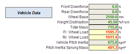
VEHICLE INPUT Data
|
The critical vehicle data, essential for determining the ride behavior of the vehicle, include Vehicle Mass, Weight Distribution, Wheelbase, and Pitch Inertia as indicated on the left.
The Pitch Inertia of the Sprung Mass is automatically calculated based on a generic x-distance deduction of the Steiner part of the Unsprung Masses relative to the Center of Gravity of the overall Vehicle Pitch Inertia. |
To accurately represent aerodynamic vehicles, a constant static downforce can be defined, ensuring the correct calculation of contact patch loads.
ROAD INPUT SIGNAL
As of RELEASE 8.0, DYNATUNE-XL STM provides a total of four different types of road input signals, each commonly used in the automotive industry for understanding and optimizing the ride oscillation of a vehicle.
The first two signals are specifically developed for frequency domain analysis, while the other two are commonly used for time domain analysis. All signals can be adjusted in amplitude and time/frequency behavior, and if desired, can be applied to one or two axles of the vehicle.
The first two signals are specifically developed for frequency domain analysis, while the other two are commonly used for time domain analysis. All signals can be adjusted in amplitude and time/frequency behavior, and if desired, can be applied to one or two axles of the vehicle.
FREQUENCY DOMAIN SIGNALS
|
TIME DOMAIN SIGNALS
|
|
2 Input Signals are available:
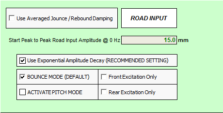
These signals are typically utilized on a 4 Poster Hydraulic Rig and can be executed in Bounce Mode or Pitch Mode. Thanks to the sinusoidal wave content, the results can be post-processed using Fast Fourier Transformations.
The Linear Decaying Sweep Sine Function is representing a road signal with Linear changing Frequency Content (typically from 0Hz to 100Hz) and if desired, changing amplitude. The signal is typically used on a 4 Poster Hydraulic Rig and can be executed in Bounce Mode or Pitch Mode. Due to the sinusoidal wave content, the results can be post-processed with Fast Fourier Transformations.
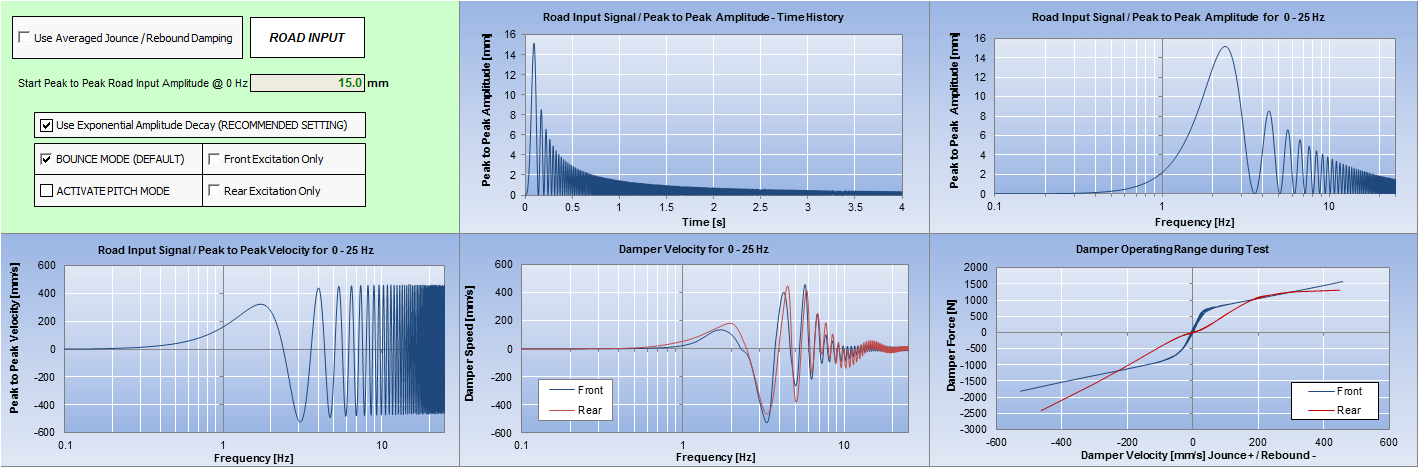
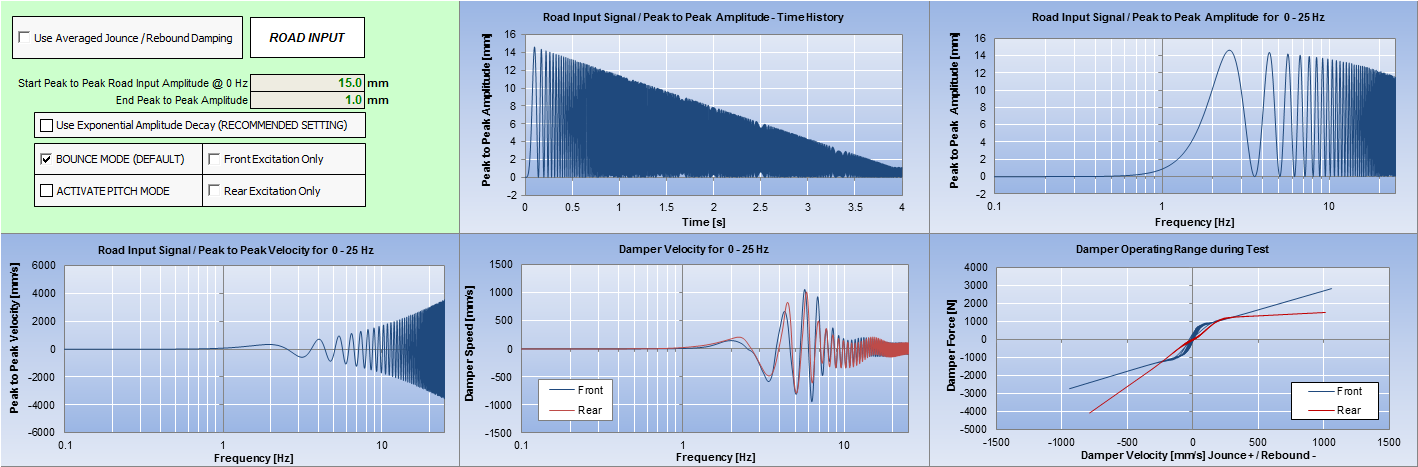
The Exponential Decaying Sweep Sine Function represents a more artificial road input signal with exponentially changing amplitude content. The key feature of such a signal is the capability of creating an input signal with CONSTANT VELOCITY, allowing for fine-tuning of the dampers in specific operating ranges.
|
2 Input Signals are available:

The Ramp/Step Function represents in effect a smooth 1/4 sinusoidal oscillation/step to a user defined Ramp Height. By setting the Ramp Length and Height & Vehicle Velocity, the Frequency Content of the Ramp is defined and displayed.
The HavSin Function represents a smooth 1/2 sinusoidal oscillation/step to a user-defined height, allowing the investigation of the vehicle's response to this input. By setting the length and height of the object and vehicle velocity, the frequency content is defined and displayed. This particular information will help the user relate the results from the HavSin Test better to the results from the Sweep Sine Test.
The HavSin Function is particularly useful for KERB Strike Events.
|
At this point it is worthwhile to mention that the Exponential Decay Signal does allow the Post Processing of Data for NON-LINEAR (Knee-Points - Strongly Different Bump and Rebound) Damper Curves. In the previous version of STM, the Fast Fourier Transformation (creating the Transfer Function) was forced to be solely executed with the averaged Jounce & Rebound Damping, mainly due to the fact that the Linear Decay Signal does contain at Higher Road Signal Input Frequencies more "Energy" than the Exponential Decaying Signal. This new signal is a major step forward towards more in-depth analyzing Non-Linear Spring/Damper Systems.
CONTROL PANEL WITH SCALING FACTORS

After entering all vehicle and suspension data and selecting the various road inputs, the user can optimize the suspension settings in the "Control Panel" by adjusting the Scaling Factors for Front and Rear Spring Rates and Jounce and Rebound Damper Characteristics. The "Live Feedback" of the most important results, all located directly around the control panel, makes it easy to explore alternatives and work towards the best compromise.
Automatic damper curve GENERATION & optimization feature
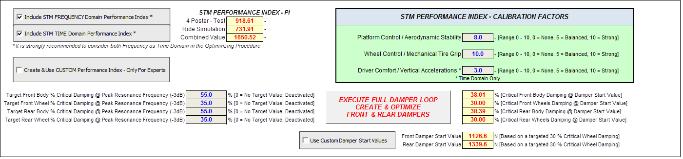
Instead of running many manual iterations towards an optimized damper setting, STM now allows for a Fully Automatic Loop, creating a suitable damper curve for the selected test events in the first step and optimizing the overall, bump, and rebound damping rates in the second step. The user can define start damping values for this process.
To create and optimize a damper curve, a proprietary Cost Function, called STM Performance Index, has been defined. It consists of a mix of Key Performance Indicators (KPIs) describing the overall "Performance" of the vehicle. Expert users can define a CUSTOM Performance Index with their own Cost Function, providing maximum tuning flexibility.
The optimization can be executed for the Frequency Domain only (4-Poster Test) or include the Time Domain (Ride Obstacle Event Simulation).
Furthermore, depending on the actual operating conditions of the vehicle, one can "Scale" the importance of three attributes in the optimization dire from 1 to 10. These three attributes are:
In addition to the FULL Automatic Loop, each of the steps can be executed manually. This allows partial optimization of damper data and the execution of repeat loops for ultimate in-depth fine-tuning.
To create and optimize a damper curve, a proprietary Cost Function, called STM Performance Index, has been defined. It consists of a mix of Key Performance Indicators (KPIs) describing the overall "Performance" of the vehicle. Expert users can define a CUSTOM Performance Index with their own Cost Function, providing maximum tuning flexibility.
The optimization can be executed for the Frequency Domain only (4-Poster Test) or include the Time Domain (Ride Obstacle Event Simulation).
Furthermore, depending on the actual operating conditions of the vehicle, one can "Scale" the importance of three attributes in the optimization dire from 1 to 10. These three attributes are:
- Platform Control for vehicles dominated by aerodynamics.
- Wheel Control for vehicles dependent on mechanical tire grip.
- Driver Comfort & Vertical Accelerations.
In addition to the FULL Automatic Loop, each of the steps can be executed manually. This allows partial optimization of damper data and the execution of repeat loops for ultimate in-depth fine-tuning.
RESULTS
STM does provide 4 Main Area's of Analysis & Results:
- Frequency Domain Analysis & Results
- Time Domain Analysis & Results
- Automatic Damper Generation & Optimization Results
- Classic Analytical & Ride Metrics
FREQUENCY DOMAIN RESULTS
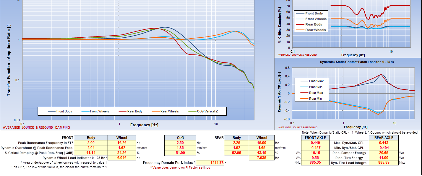
THE SWEEP SINE RESULTS consist out of 3 Main Graphs and several Performance Metrics, all in the Frequency Domain
GRAPHS:
The Frequency Transfer Function describes the relationship between the Road Input Signal and the response of the Wheels & Body to this input. It basically shows that if the road input at a frequency of 3 Hz is, for example, 10 mm, the Front Body would react with approximately 10 mm x 2 = 20 mm vertical displacement. At a frequency of 10 Hz, the Front Body would react with approximately 10 mm = 0.3 = 3 mm displacement. The presentation of such a chart representing the Frequency Domain is typically in a logarithmic scale for both the x-axis and y-axis.
This graph is, in fact, a presentation of the Percentage Critical Damping over the Frequency Spectrum. It shows the percentages of Critical Damping for Wheels and Body for a given amplitude input and excitation frequency. This allows a good overview of the amount of damping in the system over the whole operating range.
A graph displaying the "Normalized Dynamic Wheel Load" for a given excitation frequency. This is the ratio of dynamic wheel load to static wheel load, and when this value goes below -1, the wheel would, in real life, lose contact with the road. The graph allows for a quick check to see if the road signal is suited for the vehicle. Conversely, the graph shows at which excitation frequency the wheels would start losing contact with the ground for the given road input signal.
METRICS:
The Key Performance Indicators/Metrics are:
FREQUENCY DOMAIN PERFORMANCE INDEX:
The performance index combines a range of frequency domain key performance indicators (KPIs) into a cost function that can be minimized by the automatic optimization procedure.
GRAPHS:
- The Frequency Transfer Function Graph for Body & Wheel Movements.
The Frequency Transfer Function describes the relationship between the Road Input Signal and the response of the Wheels & Body to this input. It basically shows that if the road input at a frequency of 3 Hz is, for example, 10 mm, the Front Body would react with approximately 10 mm x 2 = 20 mm vertical displacement. At a frequency of 10 Hz, the Front Body would react with approximately 10 mm = 0.3 = 3 mm displacement. The presentation of such a chart representing the Frequency Domain is typically in a logarithmic scale for both the x-axis and y-axis.
- 0.1 Hz Moving Average Percentage Critical Damping
This graph is, in fact, a presentation of the Percentage Critical Damping over the Frequency Spectrum. It shows the percentages of Critical Damping for Wheels and Body for a given amplitude input and excitation frequency. This allows a good overview of the amount of damping in the system over the whole operating range.
- Dynamic Wheel Load Graph
A graph displaying the "Normalized Dynamic Wheel Load" for a given excitation frequency. This is the ratio of dynamic wheel load to static wheel load, and when this value goes below -1, the wheel would, in real life, lose contact with the road. The graph allows for a quick check to see if the road signal is suited for the vehicle. Conversely, the graph shows at which excitation frequency the wheels would start losing contact with the ground for the given road input signal.
METRICS:
The Key Performance Indicators/Metrics are:
- Dynamic Overshoot & Percentage Critical Damping Factors for Front & Rear Body at Resonance Frequency.
- Dynamic Wheel Load Indicator which does describe how close the Wheel Transfer Function remains to the Value "1".
- Maximum Dynamic / Static Contact Patch Load Ratio.
- Dissipated Energy in Dampers & Tires During The Test.
- Integrated Dynamic Tire Load over Frequency Range.
FREQUENCY DOMAIN PERFORMANCE INDEX:
The performance index combines a range of frequency domain key performance indicators (KPIs) into a cost function that can be minimized by the automatic optimization procedure.
Time DOMAIN RESULTS
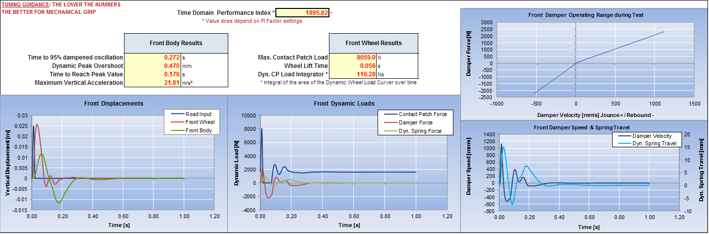
THE RAMP SINE / HAVSIN INPUT RESULTS consist out of 4 Graphs and several Performance Metrics, all in the Time Domain.
GRAPHS:
METRICS:
BODY:
WHEEL:
TIME DOMAIN PERFORMANCE INDEX:
The performance index combines a range of time domain key performance indicators (KPIs) into a cost function that can be minimized by the automatic optimization procedure.
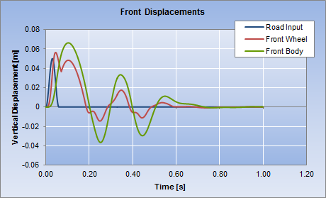
NOTE: From RELEASE 8.0 onward, in the time domain analysis, the ride model permits the wheel to lift off. The car can actually "jump." Performance metrics are divided into body and wheel key performance indicators (KPIs). All body-related KPIs describe objective measures for judging/describing the time behavior of the oscillation. The maximum vertical acceleration can be used for trade-offs or to assess comfort aspects of variants.
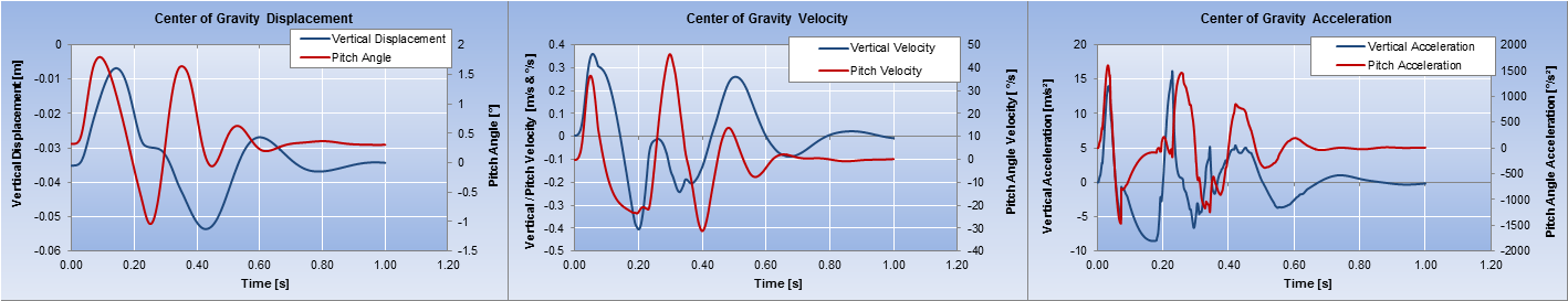
Last but not least there the tool does contain graphical representation of Accelerations, Velocities and Displacements for the Center of Gravity.
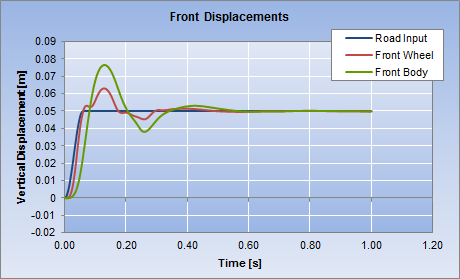
GRAPHS:
- Time Trace of Displacements for Road, Wheel & Body
- Time Trace of Dynamic Contact Patch Load, Spring & Damper Forces
- Damper Operation Points
- Time Trace of Dynamic Spring Deflection & Damper Velocity
METRICS:
BODY:
- 95% Decay Time
- Dynamic Overshoot
- Time to Reach Peak Overshoot
- Maximum Vertical Acceleration
WHEEL:
- Max / Min Contact Patch Load
- Contact Patch Load Integral
- Wheel Lift Time
TIME DOMAIN PERFORMANCE INDEX:
The performance index combines a range of time domain key performance indicators (KPIs) into a cost function that can be minimized by the automatic optimization procedure.
NOTE: From RELEASE 8.0 onward, in the time domain analysis, the ride model permits the wheel to lift off. The car can actually "jump." Performance metrics are divided into body and wheel key performance indicators (KPIs). All body-related KPIs describe objective measures for judging/describing the time behavior of the oscillation. The maximum vertical acceleration can be used for trade-offs or to assess comfort aspects of variants.
Last but not least there the tool does contain graphical representation of Accelerations, Velocities and Displacements for the Center of Gravity.
DAMPER CURVE GENERATION & OPTIMIZATION RESULTS
As mentioned above the Results of the Damper Generation & Optimization Feature can be devised into 2 Sections:

In Section 1, all results are displayed for the newly created damper curve. Step 1 presents the linear damper data, and in Step 2, one can evaluate the added knee-point characteristics. In each step, the Performance Index Graph shows the progress of the optimization process "live," and data will be "frozen" at the end of the execution of each step.
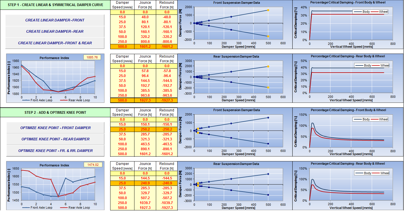

In Section 2, all results are displayed for the newly created and fully optimized damper curve. Step 3 presents the results for the optimized overall % critical damping (damping ratio), and in Step 4, one can evaluate the best combination of bump and rebound damping. As the Fast Fourier Transformation in the Frequency Domain primarily considers the total amount of damping in the system, the optimization towards bump and rebound damping is entirely executed in the Time Domain.
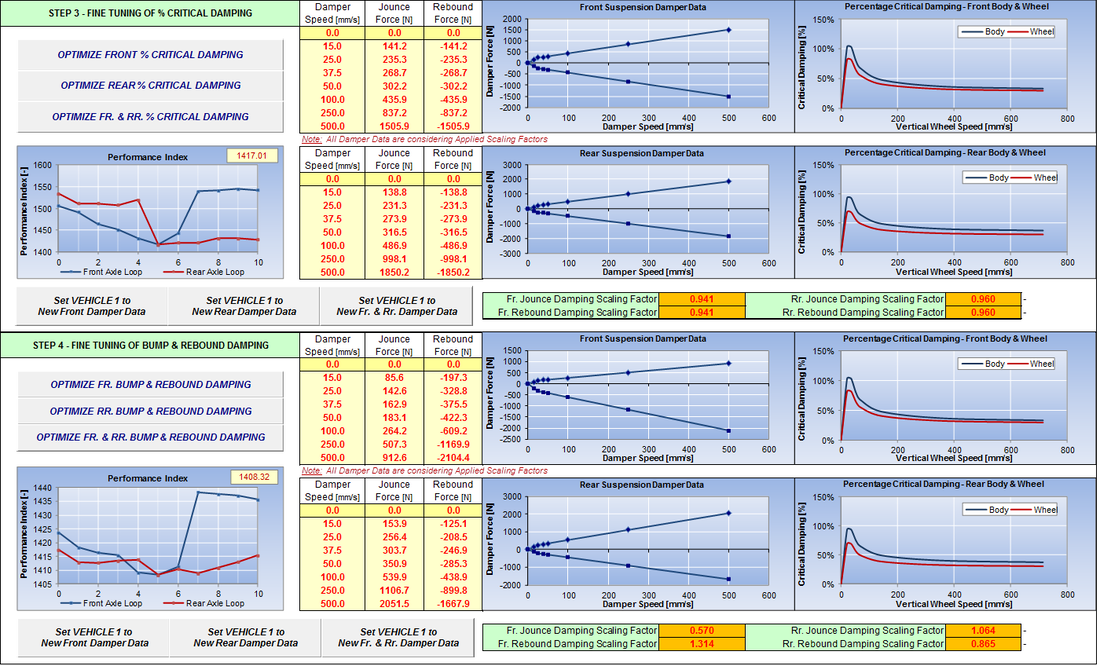
Section 2 data will be generated by scaling damper data created by Section 1 or existing damper data in the Vehicle 1 Sheet. At the end of the optimization process, the user can decide whether to set the new damper curves as new base curves.
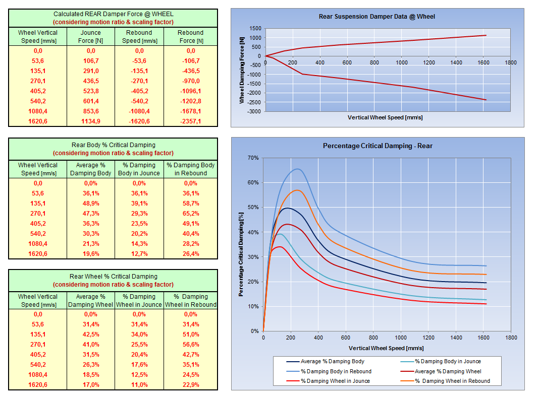
CLASSIC ANALYTICAL RESULTS
|
DYNATUNE-XL STM provides all the "Classic Literature" information on front and rear ride frequencies, percentage critical damping charts for both "Jounce" and "Rebound" damper velocities, corrected by motion ratios and scaling factors if applicable. Plots are available for both body and wheel damping.
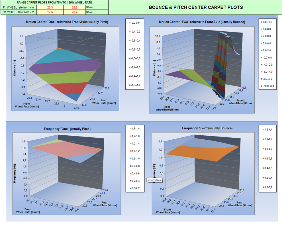
Additionally, DYNATUNE-XL STM calculates the location of the "Bounce" and "Pitch" Centers. To further optimize the vehicle setup, Carpet Plots are offered, illustrating the effects of various front and rear wheel rate combinations on the location of these centers with respect to the front axle of the vehicle. |

|
|
|
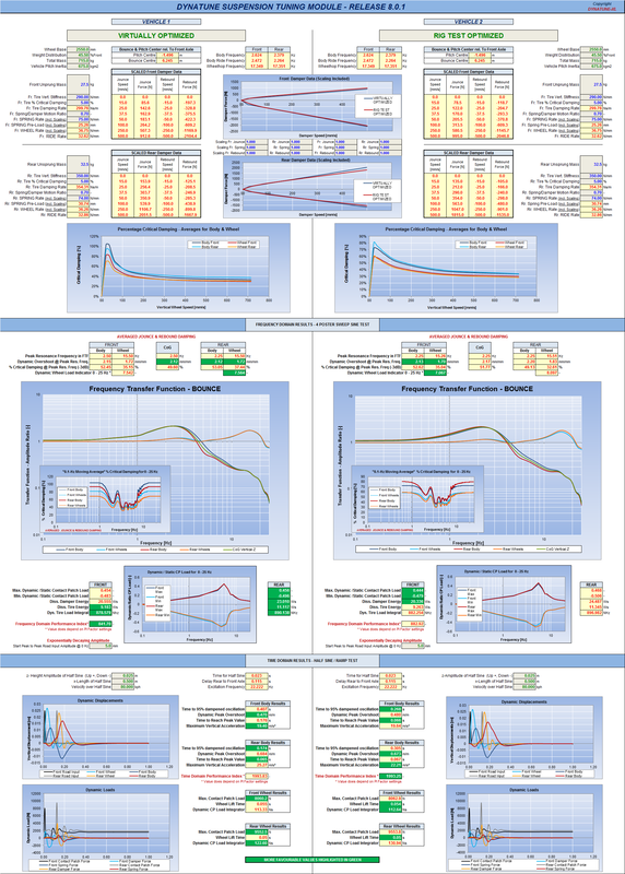
COMPARISON OF RESULTS
The Workbook does contain also a COMPARISON Sheet in which all key Parameters and Graphs for 2 Vehicles are listed allowing an easy back to back comparison of variants. Metrics which are more favorable are high-lighted in Green.